Making Neural Speech Codecs Robust to Noise with Denoising Training
Related Posts
- Overview:日本語音声基盤モデルをスケーリングさせ、TTS性能を見てみる
- Preprocessing:音声データを処理する前処理パイプラインと実行基盤を作った話
- Pre-training:日本語音声基盤モデルの事前学習
- Post-training:日本語音声基盤モデルの事後学習:TTSに強化学習を適用する
- Codec:This post
Discrete speech tokens have become a popular choice for spoken language models (SLMs) in recent years. In this article, “SLMs” means language models that can understand human speech and respond in speech to hold a conversation; they are often adapted from text LLMs. Because discrete speech tokens work like text tokens, they make it relatively easy to adapt existing LLMs to speech and train them 1, 2. Neural audio codecs (NACs) are commonly used to convert speech waveforms into such tokens. Although NACs were originally developed for audio compression, they have quickly grown beyond this purpose and become one of the most fundamental components of the SLM ecosystem.
An NAC compresses speech into a sequence of discrete tokens. An SLM takes the encoded tokens of the user’s speech to understand what they say, and the tokens it generates are mapped back to speech by the NAC’s decoder. As a compressor, the NAC is expected to reconstruct speech faithfully and in high quality, so that the SLM output sounds good. At the same time, the NAC serves as a bridge from raw, continuous, and often noisy recordings to abstract, discrete linguistic content that supports downstream language modeling tasks. If the NAC already extracts this content well and makes it accessible in its tokens, the downstream model can understand it more easily.
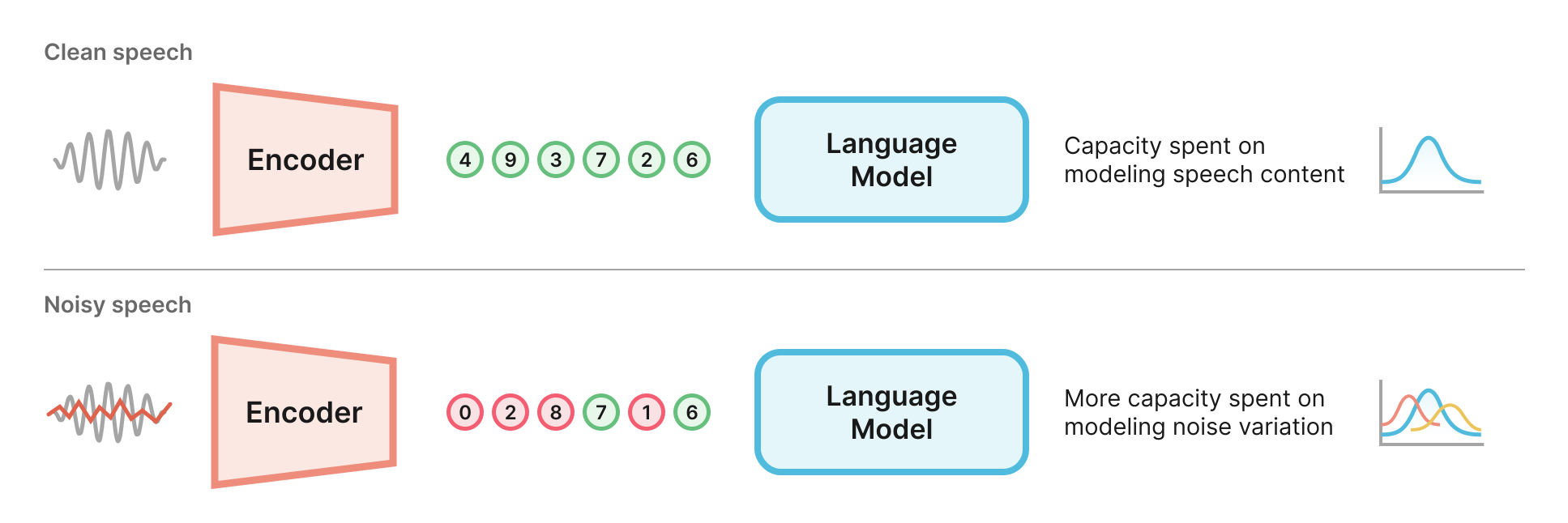
Noisy speech introduces more variance on tokens, reducing useful linguistic information; downstream language model wastes its capacity to model that variance.
However, during this conversion, noise can significantly affect the performance of NACs and the quality of the extracted linguistic information. Users record their voices with different devices and microphones, in different environments and situations. These can range from a cafe in the morning with soft background babble to a downtown street at rush hour near a construction site. Many have found that the performance of SLM systems degrades in such noisy real-world conditions 3, 4, 5. In our internal evaluation, a naive full-duplex SLM was so sensitive that even changing user’s microphone affected its performance. Therefore, to support a strong conversational AI system, speech tokenization should be robust to such noise.
In this article, we describe how we tackle this problem by training a noise-robust NAC.
Basics of Neural Audio Codec
Before getting to our design, let’s review the basics of NACs. An NAC is usually implemented as a VQ-VAE (vector-quantized variational autoencoder), which compresses a waveform into latents that can be turned into discrete tokens. A typical NAC recipe contains these ingredients:
- Model backbone. An encoder-decoder mechanism, usually based on convolutional neural networks (CNNs) or Transformers, is used to map a waveform into a sequence of embeddings and vice versa.
- Quantizer. A quantizer discretizes the continuous latent embeddings into a sequence of discrete IDs.
- GAN training. In addition to the essential reconstruction objective, GAN training is often added to enhance generation fidelity. A discriminator is trained simultaneously to tell apart reconstructions from real audio; the codec (as generator) is trained to deceive the discriminator.
- Teacher model for knowledge distillation. Pure autoencoder training is not ideal for extracting useful linguistic information. A popular way to improve this is to distill knowledge from pretrained self-supervised learning (SSL) models 2, 6, 7, such as WavLM 8 and w2v-BERT 2.0 9, whose embeddings have been shown to capture prominent phonetic structure 10. This is not strictly necessary, but can be important when the compression rate is high.
- Losses: reconstruction losses, GAN losses, distillation losses, and sometimes quantizer losses.
In this article, we use MOSS-Audio-Tokenizer as our baseline for both development and evaluation, since it achieved the best performance in our internal evaluation. It uses a fully transformer-based backbone with causal sliding window attention, where down- and up-sampling are implemented by patchify (reshape) operations. It uses Residual Vector Quantization (RVQ) and produces 16–32 layers of 12.5Hz tokens (with a vocabulary size of 1024). It comes with two variants: Base (1.6B parameters) and Nano (22M parameters).
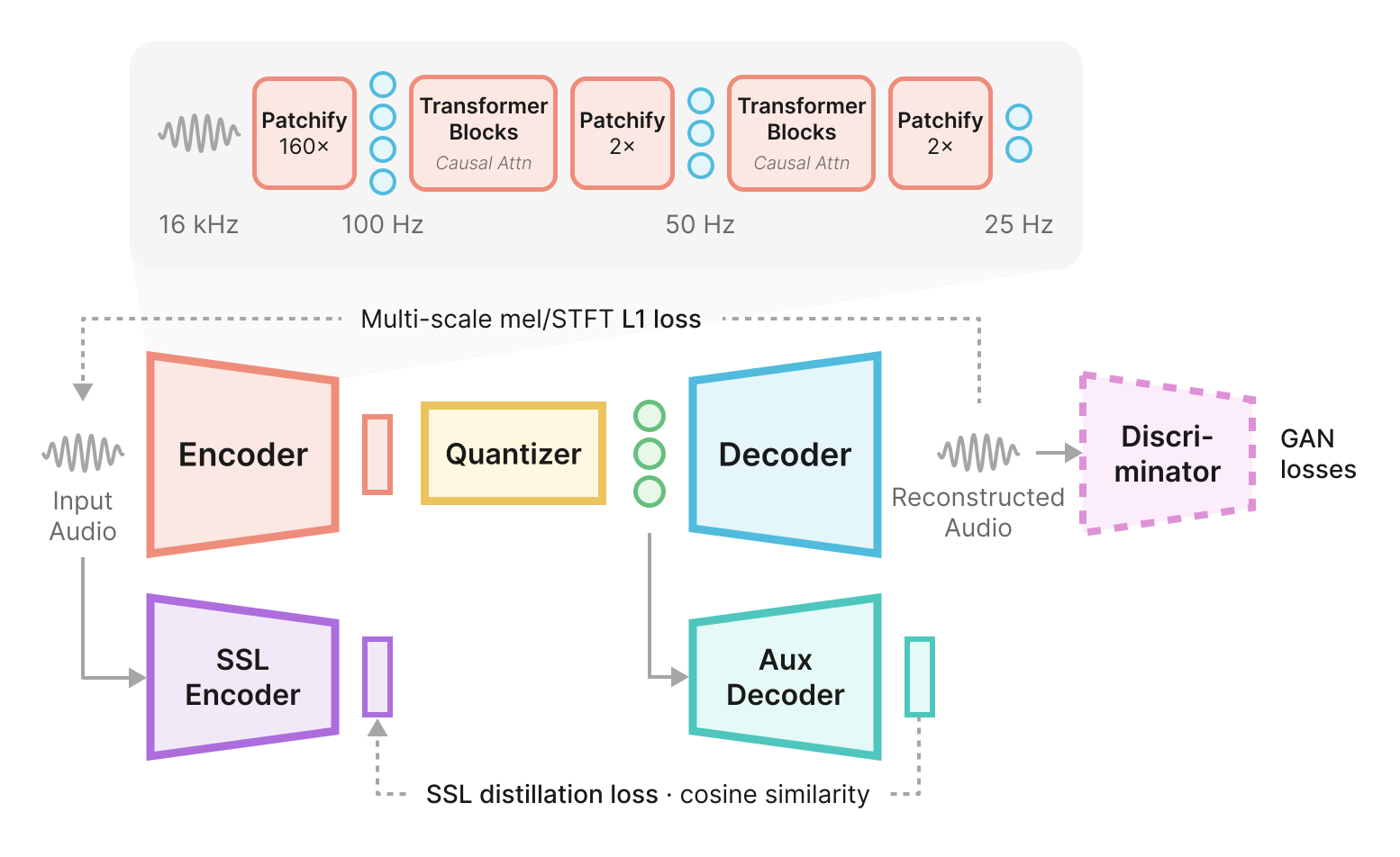
Architecture of our base model.
Inspired by MOSS-Audio-Tokenizer, we design a base model for our experiments. Since longer token sequence will take transformer-based SLMs longer to train, we aim at a lower token rate. To lower the token rate and simplify training, we use a non-parametric quantizer (one without a learned codebook) to produce a single stream of 25Hz tokens (with a vocabulary size of ~50k, resulting in ~390 bits per second). Instead of applying distillation loss on RVQ codes, we use an auxiliary decoder to predict SSL features from our single-layer codes. The model has 260M parameters (not counting training-only components). We denote it as “Ours (base)” below.
In the experiments, to bring MOSS-Audio-Tokenizer close to our bitrate, we take the first 2 or 4 layers of their tokens, resulting in 250 or 500 bits per second (25 or 50 tokens per second), respectively. We denote them as “MOSS-Nano/Base q2/q4”.
What changes with noise?
To quantify the problem, we analyze how encoded tokens and reconstructions change as noise gets stronger. We use LibriTTS-R test-clean (English) 11 and JVS (Japanese, randomly sampled to 5 hours) 12 as our evaluation sets, and add random noise to them at controlled signal-to-noise ratios (SNRs). The noise files are sampled from the following environmental sound datasets: AudioSet, FSD50K, WHAM!, and DEMAND (clips with clear human sounds or music are excluded to avoid interfering with the speech content). Both the clean and noisy (at different SNR levels) data are then encoded and reconstructed by each codec.
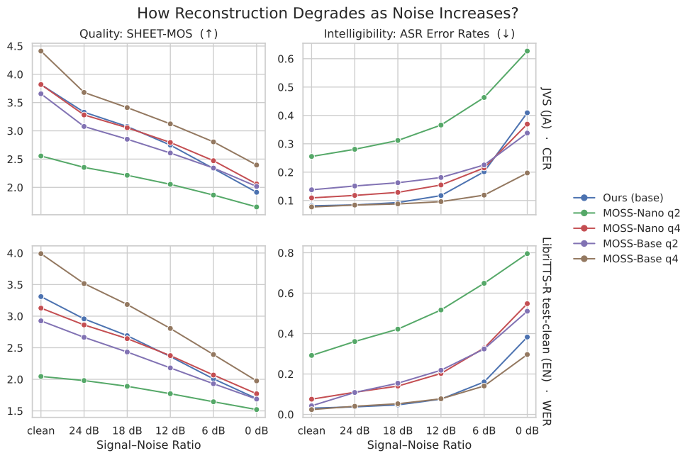
How does objective reconstruction metrics degrade as input noise increases? For intelligibility results, CER is used for Japanese, WER is used for English.
First, we calculate objective metrics on reconstructions to see how well the models can recover essential information from noisy speech. In the two plots on the left, the neural quality score (SHEET-MOS) 13 results show that reconstruction quality degrades as noise gets stronger (lower SNR). On the right, the intelligibility results, calculated with existing ASR models (word error rate (WER) by parakeet-tdt-0.6b-v2 for English, and character error rate (CER) by parakeet-tdt_ctc-0.6b-ja for Japanese), show that it becomes harder to correctly transcribe the spoken content from the reconstructions. In other words, the extracted linguistic content is being corrupted by the added noise. At an SNR of 6dB, the WERs of some models already draw near to 20%. With larger models and more tokens, the degradation is less severe. The performance of our base model (390bps, 25 tokens/s, 260M) falls roughly between MOSS-Base q4 (500bps, 50 tokens/s, 1.6B) and MOSS-Nano q4 (500bps, 50 tokens/s, 22M).
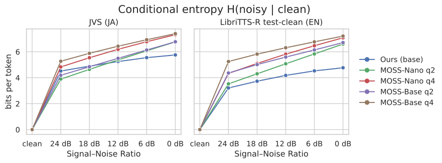
How much uncertainty does noise add to tokens?
Next, we look at the encoded tokens directly to see how they change with stronger noise. From the perspective of downstream language modeling, what matters is not which token IDs change, but how much the tokens vary. If the tokens vary more after noise is added, the SLM has to use more capacity to model those variations, and will likely be more susceptible to noise.
To measure this, we encode each utterance twice, once clean and once with added noise. Since adding noise does not change the length of the audio, the two token sequences are aligned frame by frame. For a codec with $L$ codebook levels ($L = 1$ for ours; $L = 2$ or 4 for MOSS q2/q4), let $C_\ell$ and $N_\ell$ be the level-$\ell$ tokens at the same frame from the clean and noisy speech. Counting these pairs over all frames in the evaluation set gives an empirical distribution $p(c, n)$, from which we compute the conditional entropy for each level and average over levels:
$$ \begin{aligned} H(N_\ell \mid C_\ell) &= -\sum_{c,\,n} p(c, n) \log_2 \frac{p(c, n)}{p(c)}, \\ \bar{H} &= \frac{1}{L} \sum_{\ell=1}^{L} H(N_\ell \mid C_\ell). \end{aligned} $$$H(N_\ell \mid C_\ell)$ is the average number of bits still needed to know a noisy token once the clean token at the same position is known. That is, how many bits of uncertainty noise adds per token. If noise never changes the tokens, it is 0. It is also 0 if noise always turns a given clean token into the same other token, since such a consistent change is easy to learn. It grows when the same clean token can turn into many different noisy tokens. We use it as a proxy for how much extra variation noise brings into the token stream for a downstream LM to model.
In the figure, we can see that for all models, the conditional entropy increases as noise gets stronger. Within the RVQ baseline, using more levels raises the average, which means the higher levels change more under noise than the lower ones. This matches the common view that higher RVQ levels capture finer acoustic variations. Interestingly, MOSS-Base shows higher entropy than MOSS-Nano. This might indicate that the larger model captures more acoustic variation with the same token capacity to improve reconstruction, which in turn leads to worse noise robustness in token space.
The results above confirm our suspicion from the introduction: standard NACs are indeed sensitive to noise, and the performance of downstream SLMs will probably degrade in noisy conditions. This is because the codecs include irrelevant variations in their token space, which wastes the downstream LM’s capacity to model them.
A simple approach: Augment and Denoise
Making a speech encoder robust to noise largely means making it produce representations that are invariant under different acoustic conditions. In the training of many SSL models, including speech models such as WavLM 8 and w2v-BERT 2.0 9, the data is augmented into different versions, and the model is asked to produce similar embeddings for them (as in contrastive learning) or to predict labels derived from the original data (as in masked prediction). In this way, the encoder learns to capture the invariant structure in the data and ignore the variation.
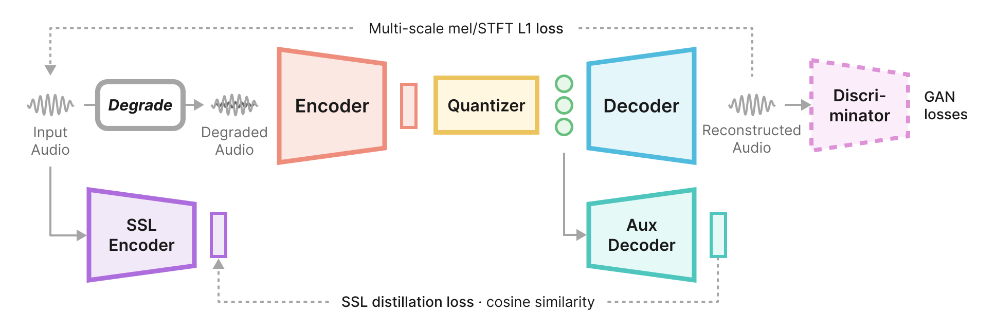
Architecture of our denoising model. The model predicts clean speech and clean SSL features from degraded audio.
We can naturally apply this idea to our codec: augment the input data with noise, then ask the model to predict the original clean data. In the SSL distillation branch, we also ask the auxiliary decoder to predict the SSL features extracted from the original data 7. The clean audio and features act as anchors that encourage the model to learn invariant representations.
This denoising codec formulation is in fact very similar to speech enhancement/restoration models, such as Miipher 14 and Sidon 15, which also take degraded speech as input and predict the original clean speech. However, those models often use existing SSL embeddings as their internal representations and train the encoder and decoder (vocoder) separately, while our denoising codec needs to learn its own representations end-to-end. Our codec also operates under a relatively tight bitrate budget. Because of these differences, a denoising codec probably needs less aggressive augmentation.
To summarize at a high level: on the encoder side, the model is trained to produce representations that are invariant to augmentation, similar to robust SSL models; on the decoder side, the model is trained to restore degraded audio to clean audio, similar to speech enhancement models. Together, this formulation encourages the model to be robust to noise on both the input and output sides.
The degradation pipeline
To design a degradation method that simulates real-world effects, we consider several broad aspects:
- Room acoustics: The size, shape, material, etc. of a room can affect how sound is finally heard.
- Ambient noise: Other sound sources can distract listeners from the speaker. Noises can differ greatly in acoustic characteristics and dynamics, ranging from a quiet fan hum to a loud dog bark.
- Microphone type: Different microphones have different frequency responses and recording qualities, which can color the sound differently or even degrade it.
- Encoding and transmission errors: Digital audio processing and transmission can introduce artifacts, such as clipping, band limiting, and unexpected interruptions.
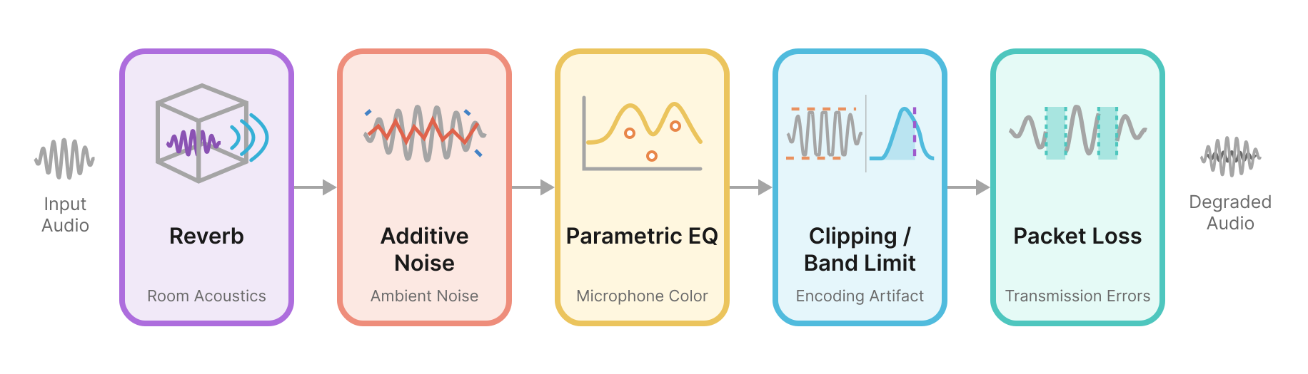
Our audio degradation pipeline for augmented training.
These aspects are not independent and are often mixed together in real recordings. Following the rough order in which they happen, we design a degradation pipeline that simulates these real-world effects during training.
Our implementation refers to several works on robust SSL and speech enhancement (Sidon 15, WavLM 8, XEUS 16, Gat et al. 17, NAST 18). Based on the intuitions above, the stages of our pipeline are as follows:
-
Reverb: When sound travels in a room, the microphone receives the direct sound plus many delayed, weakened echoes reflected from walls, floors, and objects. These sounds form reverberation. Reverb can be described by a room impulse response (RIR), which records how a particular room responds to a single click. Convolving clean audio with an RIR makes it sound as if it were recorded in that room.
Our RIRs are drawn 50/50 from two sources: (1) real RIRs from the Room Impulse Response and Noise Database, and (2) on-the-fly simulated RIRs usingpyroomacousticsshoebox simulation. The convolved audio is then re-aligned to remove the delay caused by the RIR, which is estimated from the RIR’s peak position. -
Additive noise: Ambient noise is simply mixed with the speech signal. Its strength is measured by the signal-to-noise ratio (SNR), the energy ratio between speech and noise in decibels. Higher SNR means cleaner speech; lower SNR means louder noise.
Our noise samples are drawn 85/15 from two sources: (1) a real recorded noise corpus, and (2) on-the-fly simulated wind noise using SC-Wind-Noise-Generator. The noise corpus includes 4 datasets: AudioSet, FSD50K, WHAM!, and DEMAND (clips with clear human sounds or music are excluded to avoid interfering with the speech content). A noise sample is randomly cropped to 0–100% of the original segment length (looped if shorter), then added at a random position with a random SNR between 12 and 30dB. -
Parametric equalization (EQ): A microphone’s frequency response determines how strongly it picks up each frequency, so different microphones emphasize or suppress different parts of the spectrum. An equalizer reproduces this effect by raising or lowering specific frequency regions with a combination of filters: (1) pass filters remove frequencies beyond a point; (2) shelf filters raise or lower all frequencies above or below a point; (3) peak filters raise or lower a narrow band around a center frequency.
Implementation details
Our EQ includes a low end, a high end, and 8 peaks in the middle. The low end (logarithmically sampled from 20–500Hz) is randomly chosen from a low-shelf or a high-pass 50/50; similarly, the high end (logarithmically sampled from 3–8kHz) is chosen from a high-shelf or a low-pass. The shelf filters are maximally flat and choose a gain uniformly from -6 to 6dB. The pass filters are also maximally flat and choose from 12/18/24 dB/oct slopes. The peak filters are evenly distributed in the log frequency space of 100–6000Hz, each has uniformly sampled gain from -6 to 6dB and Q factor from 2–6.
-
Clipping: A recording or a processing stage often has a maximum amplitude it can handle. When the input is too loud, the waveform peaks are flattened at that limit. This sounds like a distortion effect.
To randomize the intensity, we pick a high cutoff from the 95–100th amplitude percentile and also a low cutoff from the 0–5th, then clamp the waveform using those thresholds. -
Band-limit: Telephone systems often use 8kHz sampling, which gives speech a muffled quality. We simulate this by resampling audio to 8kHz and back to the original rate.
-
Packet loss: To simulate network instability, we zero out 10–50ms bursts at random positions, covering at least 5% of the audio.
Each stage is applied independently with a probability of 50%, so the combinations are more diverse. Since the model still needs to handle clean input, 50% of the training samples are kept clean.
Here are some samples showing the effect of each degradation stage (many of the effects are easy to see in the spectrograms):
| Degradation | Spectrogram | Audio |
|---|---|---|
| Original | 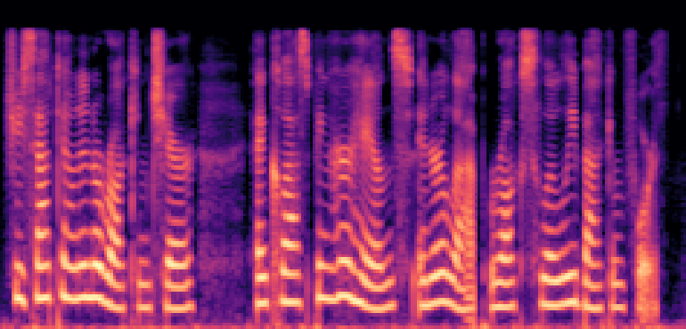 |
|
| Reverb | 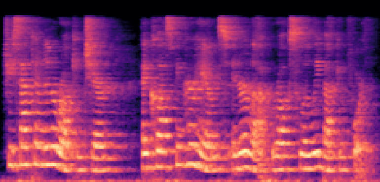 |
|
| Additive noise | 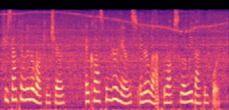 |
|
| Parametric EQ | 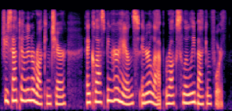 |
|
| Clipping | 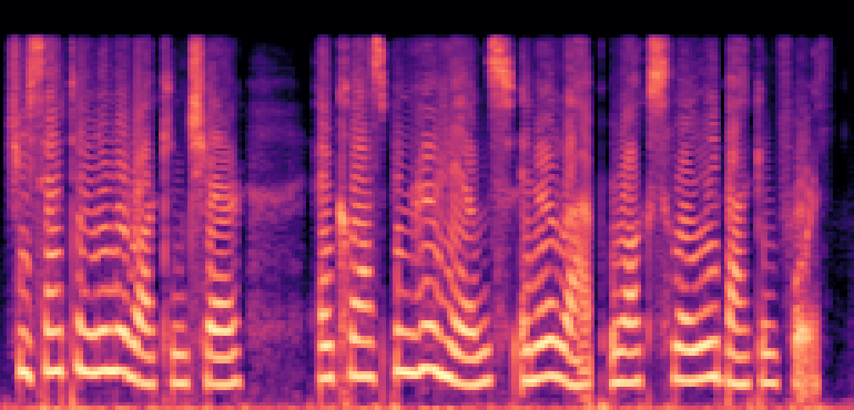 |
|
| Band-limit | 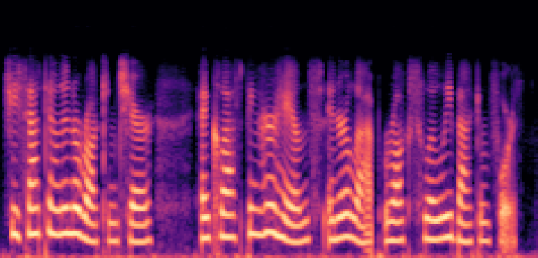 |
|
| Packet loss | 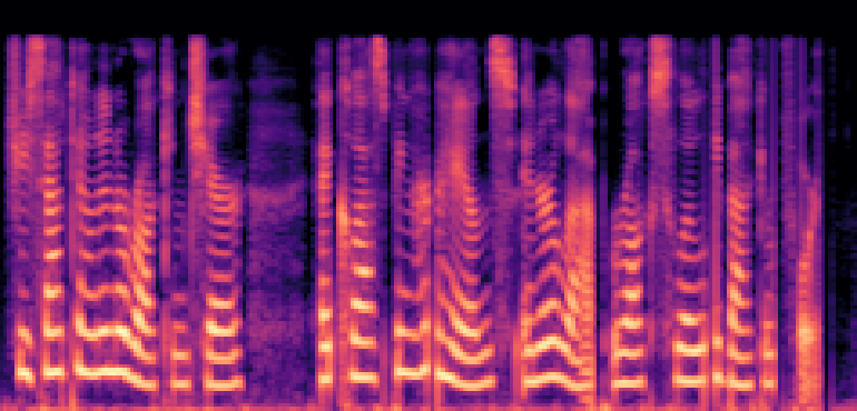 |
|
| Everything combined | 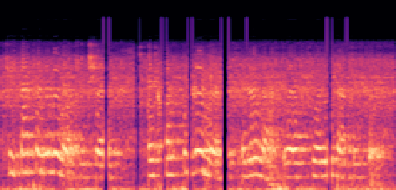 |
Results
We show some reconstruction samples of noisy audio. We can hear that the MOSS models try to include the noise in their reconstructions, which hurts the quality, while our denoising model reduces the noise and keeps the linguistic content.
| Model / input | LibriTTS-R (English) | JVS (Japanese) |
|---|---|---|
| Noisy input (SNR = 12 dB) | ||
| Ours (base) | ||
| Ours (denoising) | ||
| MOSS-Nano q2 | ||
| MOSS-Nano q4 | ||
| MOSS-Base q2 | ||
| MOSS-Base q4 |
Next, we apply the same evaluations from the previous section to our denoising model, denoted as “Ours (denoising)” in the figures (orange lines). The results of the other models remain the same.
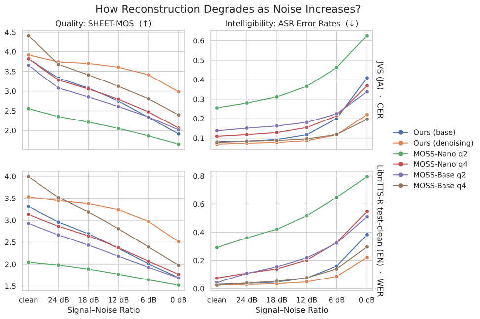
How does objective reconstruction metrics degrade as input noise increases? For intelligibility results, CER is used for Japanese, WER is used for English.
As the figure shows, Ours (denoising) generally has better quality, intelligibility, and robustness (gentler slopes) on noisy speech. Compared to Ours (base) (blue lines), the improvement is significant. Moreover, despite its lower bitrate, lower token rate, and much smaller size (390bps, 25 tokens/s, 260M) compared to MOSS-Base (500bps, 50 tokens/s, 1.6B), Ours (denoising) performs on par with or better than MOSS-Base. This shows that our denoising training framework effectively improved the model’s noise robustness.
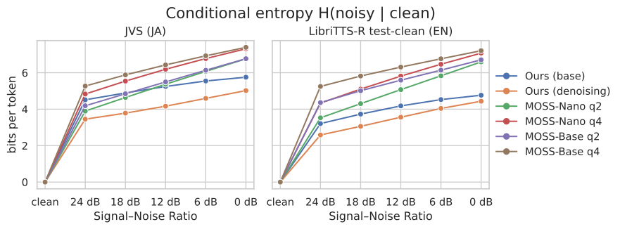
How much uncertainty does noise add to tokens?
Regarding encoded tokens, the conditional entropy of the tokens produced by Ours (denoising) is significantly lower than that of Ours (base) and the MOSS models. This shows that the uncertainty caused by noise is reduced, so the downstream model wastes less capacity on irrelevant variation. However, the slopes in the figure don’t change much, which suggests that some of the uncertainty caused by stronger noise may be intrinsic and cannot be eliminated.
Combining the two results above, we found that, in general, Ours (denoising) achieves among the best reconstruction quality and the lowest token space variation at the same time under noisy conditions. In contrast, for MOSS tokenizers, those aspects seem conflicting—better reconstruction quality (by larger model and more tokens) almost always results in worse token space variation. For example, MOSS-Base q4 achieves the best-in-class reconstructions but the highest conditional entropy; MOSS-Nano q2 gets the best conditional entropy but the worst reconstructions. This is probably because NACs trained with a standard reconstruction objective are optimized to include as many acoustic variations as possible to improve reconstruction quality. On the other hand, our denoising model is encouraged to extract linguistic information regardless of noise. Its improvement in reconstruction comes not from including more acoustic variation, but from better capturing the linguistic content. In this way, it can improve both aspects together.
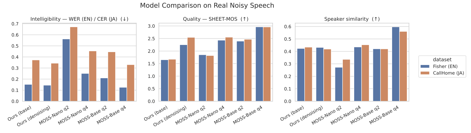
Comparison on real-world noisy speech (Fisher and CallHome Japanese).
Finally, we test the models on real-world noisy speech datasets: Fisher in English and CallHome Japanese, both containing spontaneous telephone conversations. Ours (denoising) remains competitive with MOSS-Base, especially in intelligibility, despite using fewer tokens and a much smaller model. MOSS-Base q4 is still clearly ahead in quality (SHEET-MOS) and speaker similarity.
Conclusion
In this article, we showed that standard neural audio codecs (NACs) are sensitive to noise. Their reconstruction quality and intelligibility drop, and the encoded tokens drift from the clean ones. Downstream language models have to waste extra capacity on noise variation that carries no meaningful linguistic information.
To address this, we trained our tokenizer with a simple “augment-and-denoise” objective: degrade the input with a pipeline simulating reverb, ambient noise, microphone characteristics, and encoding/transmission artifacts, then ask the model to predict clean speech and SSL features.
Our key findings are:
- Better reconstruction under noise: Our denoising model improves quality and intelligibility over our base model, and matches or outperforms MOSS-Audio-Tokenizer (Base) on our noisy evaluation sets despite a lower bitrate, lower token rate, and a much smaller model. On real-world telephone conversations (Fisher and CallHome Japanese), it remains competitive, especially in intelligibility.
- More stable information encoding under noise: The denoising model achieves the lowest conditional entropy among all models tested, meaning that noise introduces less uncertainty to the token stream.
- Quality and stability can improve together: For codecs trained with a standard reconstruction objective, there seems to be a trade-off between reconstruction quality and token stability, since models spend more capacity on acoustic variation, including noise, to improve quality. In contrast, the denoising objective encourages the model to capture useful linguistic content and discard irrelevant variation, so that both sides can be improved together.
Some questions still remain open. The degradation pipeline currently only considers speech sounds and excludes other conditions (including non-verbal expressions and background speech) and music (which often contains singing) to avoid interference, even though they are very common in real-world scenarios. Moreover, the token space analysis cannot fully replace a direct evaluation of downstream SLMs under real-world conditions, as positive upstream results do not always lead to positive downstream performance. We leave these for future work.
Related Posts
- Overview:日本語音声基盤モデルをスケーリングさせ、TTS性能を見てみる
- Preprocessing:音声データを処理する前処理パイプラインと実行基盤を作った話
- Pre-training:日本語音声基盤モデルの事前学習
- Post-training:日本語音声基盤モデルの事後学習:TTSに強化学習を適用する
- Codec:This post
References
-
D. Zhang et al., “SpeechGPT: Empowering large language models with intrinsic cross-modal conversational abilities,” in Findings of the Association for Computational Linguistics: EMNLP 2023, 2023. ↩︎
-
A. Défossez et al., “Moshi: A speech-text foundation model for real-time dialogue,” arXiv preprint arXiv:2410.00037, 2024. ↩︎ ↩︎
-
Y. Chen, X. Yue, C. Zhang, X. Gao, R. T. Tan, and H. Li, “VoiceBench: Benchmarking LLM-based voice assistants,” Transactions of the Association for Computational Linguistics, 2026. ↩︎
-
L. Zhang et al., “WildSpeech-Bench: Benchmarking end-to-end SpeechLLMs in the wild,” arXiv preprint arXiv:2506.21875, 2025. ↩︎
-
Y. Peng et al., “FD-Bench: A full-duplex benchmarking pipeline designed for full duplex spoken dialogue systems,” in Proc. Interspeech 2025, 2025. ↩︎
-
X. Zhang, D. Zhang, S. Li, Y. Zhou, and X. Qiu, “SpeechTokenizer: Unified speech tokenizer for speech language models,” in Proc. International Conference on Learning Representations (ICLR), 2024. ↩︎
-
Z. Ye et al., “Codec does matter: Exploring the semantic shortcoming of codec for audio language model,” Proceedings of the AAAI Conference on Artificial Intelligence, 2025. ↩︎ ↩︎
-
S. Chen et al., “WavLM: Large-scale self-supervised pre-training for full stack speech processing,” IEEE Journal of Selected Topics in Signal Processing, 2022. ↩︎ ↩︎ ↩︎
-
L. Barrault et al., “Seamless: Multilingual expressive and streaming speech translation,” arXiv preprint arXiv:2312.05187, 2023. ↩︎ ↩︎
-
A. Pasad, B. Shi, and K. Livescu, “Comparative layer-wise analysis of self-supervised speech models,” in Proc. IEEE International Conference on Acoustics, Speech and Signal Processing (ICASSP), 2023. ↩︎
-
Y. Koizumi et al., “LibriTTS-R: A restored multi-speaker text-to-speech corpus,” in Proc. Interspeech 2023, 2023. ↩︎
-
S. Takamichi, K. Mitsui, Y. Saito, T. Koriyama, N. Tanji, and H. Saruwatari, “JVS corpus: Free Japanese multi-speaker voice corpus,” arXiv preprint arXiv:1908.06248, 2019. ↩︎
-
W.-C. Huang, E. Cooper, and T. Toda, “SHEET: A multi-purpose open-source speech human evaluation estimation toolkit,” in Proc. Interspeech 2025, 2025. Code: https://github.com/unilight/sheet ↩︎
-
Y. Koizumi et al., “Miipher: A robust speech restoration model integrating self-supervised speech and text representations,” in Proc. IEEE Workshop on Applications of Signal Processing to Audio and Acoustics (WASPAA), 2023. ↩︎
-
W. Nakata, Y. Saito, Y. Ueda, and H. Saruwatari, “Sidon: Fast and robust open-source multilingual speech restoration for large-scale dataset cleansing,” in Proc. IEEE International Conference on Acoustics, Speech and Signal Processing (ICASSP), 2026. ↩︎ ↩︎
-
W. Chen et al., “Towards robust speech representation learning for thousands of languages,” in Proc. Conference on Empirical Methods in Natural Language Processing (EMNLP), 2024. ↩︎
-
I. Gat et al., “Augmentation invariant discrete representation for generative spoken language modeling,” in Proc. 20th International Conference on Spoken Language Translation (IWSLT), 2023. ↩︎
-
S. Messica and Y. Adi, “NAST: Noise aware speech tokenization for speech language models,” in Proc. Interspeech 2024, 2024. ↩︎